Completeness Contours

In this example we generate completeness contours from a suite of injection-recovery tests run using the rvsearch inject command

import os

import numpy as np
import pylab as pl

import rvsearch
from rvsearch.inject import Completeness
from rvsearch.plots import CompletenessPlots

Construct a Completeness object from the output of an injection-recovery run (recoveries.csv). If we want to convert to semi-major axis and msini on construction we need to pass a stellar mass.

recfile = os.path.join(rvsearch.DATADIR, 'recoveries.csv')

comp = Completeness.from_csv(recfile, 'inj_au', 'inj_msini', mstar=1.1)

Next we calculate completeness on a grid with the specified boundaries using a 2D moving average. See Howard & Fulton (2016) for a description of the moving average method.

xi, yi, zi = comp.completeness_grid(xlim=(0.05, 100), ylim=(1.0, 3e4), resolution=25)

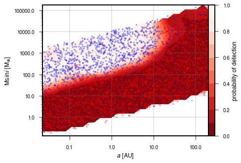
Now contruct the CompletenessPlots object and plot the contours and individual injections

cp = CompletenessPlots(comp)
fig = cp.completeness_plot(xlabel='$a$ [AU]', ylabel=r'M$\sin{i}$ [M$_{\oplus}$]')

We can also use the Completeness object to interpolate the completeness at any point in the grid.

comp.interpolate(1.0, 100, refresh=True)

array(0.32290539)